Terminators at the Terminator

The nicest thing about the word terminator is that it already sounds like a machine sent back from the future to explain your capital expenditure problem, or to make you realize the capital expenditure will not save you from a distant AI dominated dystopian doomsday.

In orbital mechanics it means something calmer and stranger: the line between day and night. A dawn-dusk sun-synchronous orbit rides that line around Earth, keeping the spacecraft in near-continuous sunlight. For Earth observation satellites this is useful because the illumination geometry stays predictable. For solar-powered orbital infrastructure it is more tempting: maximum duty cycle, fewer battery cycles, and the delicious thought that your data center can spend most of its life with the Sun on tap.

So yes, the terminators at the terminator. AI training and inference workloads running in low Earth orbit, fed by photovoltaics, cooled by radiators, and connected through optical links to ground stations and other satellites. A nice science-fiction phrase once you have solved the heat and materials balance to get up the gravity well.

The dawn-dusk sales pitch

The pitch is not silly. It starts from real constraints.

AI data centers are going to become giant electrical-to-heat converters with a side effect of model weights. Reminds me of the time when I used to dry my laundry on my bitcoin miners. On Earth we feed them through grids, substations, diesel backup contracts, cooling towers, chillers, water rights, fibre backbones, and increasingly awkward community meetings. In orbit you can imagine skipping some of that. Put the compute near continuous sunlight. Use high-efficiency solar arrays. Use direct-to-space radiators instead of evaporating water or warming a river. Place inference near space-borne sensors. Put pre-processing close to Earth observation instruments so the useful bits come down instead of the whole firehose.

NVIDIA’s Vera Rubin platform is the more immediate reference. Vera is the CPU and Rubin is the GPU, assembled with networking, memory, and rack-scale infrastructure as the successor generation to Blackwell. The roadmap promises another large increase in AI training and inference throughput, but throughput arrives with denser power delivery, cooling, and interconnect requirements. An orbital operator would inherit the useful work per watt and every unresolved watt of heat. Rubin therefore belongs in the radiator calculation as much as in the model-training benchmark.

Sensor-side inference offers a different use for that compute. The instrument looks down, the processor sits nearby, and the network carries detections, embeddings, tiles, compressed products, or model updates instead of raw sensor exhaust. A satellite constellation does not want to be a fleet of USB drives with antennas. It wants to be a distributed science platform with a power budget.

That is where dawn-dusk orbit starts to look like a scheduling primitive. Solar availability shapes the compute cluster. Training jobs, inference bursts, checkpointing, downlink windows, thermal soak, battery reserves, and radiator orientation all become part of the same planner.

The cloud scheduler gets an ephemeris.

The thermal model is the business model

On Earth, a data center engineer can cheat emotionally because air exists. It may be hot air, badly ducted air, or air pushed around by fans with punishing maintenance schedules, but it is there. You can move heat by convection. You can move it into water. You can bury part of the problem in a cooling tower plume and another part in a utility bill.

In orbit, there is no convenient atmosphere to carry the embarrassment away. Heat leaves by radiation, which puts the radiator alongside the processors and power supply in the core computer architecture.

The governing shape is brutally simple:

P = ϵσAT⁴

Radiated power depends on emissivity, area, and the fourth power of absolute temperature. Want to reject more heat without growing a ridiculous radiator? Run hotter. Want to run hotter? Your semiconductors, packages, solder joints, optics, interconnects, dielectrics, memory, and power electronics all need to tolerate it. A space data center is a semiconductor materials problem wearing solar panels.

This is why the recent attention around high-temperature semiconductors is interesting. Wide-bandgap devices such as silicon carbide and gallium nitride are already changing terrestrial power electronics because they switch efficiently and tolerate higher temperatures than conventional silicon in many roles. Push the idea further into ultra-wide-bandgap materials, diamond substrates, high-temperature packaging, and radiation-tolerant device physics, and the space qualified semiconductor variant emerges: hotter electronics can make every square metre of radiator work harder.

But that sentence hides several doctoral theses and a lot of broken hardware.

A transistor surviving a hot test coupon proves very little about the complete system. The whole compute stack has to behave: memory retention, timing margins, optical alignment, thermal cycling, electromigration, single-event effects, packaging stress, and the boring connectors that always become interesting at the worst possible time. Better high-temperature semiconductors help, but orbital data centers need a complete materials and packaging stack. A spectacular junction-temperature result does not provide one. We do not have the advanced PDK’s or foundries to do this today, but definitely a warm blue ocean of high temperature hardware to swim into.

Insulation is not the opposite of cooling

The intuitive mistake is to think space is cold, so cooling must be easy.

Space is not cold in the way a cold beer is cold. Space is mostly empty. A surface in sunlight gets blasted by roughly 1,361 W/m^2 before geometry and efficiency. A surface looking into deep space can radiate beautifully, but only if it is allowed to see deep space and only if the heat can get there.

So the architecture becomes a discipline of separation. Keep solar absorption away from the radiator side. Keep hot compute planes thermally connected to heat pipes, pumped loops, or thermal straps. Keep sensitive optics and timing hardware isolated from thermal gradients. Use multi-layer insulation where you want less radiative coupling. Use high-emissivity radiator coatings where you want more. Stop random structure from becoming a thermal short. Decide what gets to be warm, what must stay stable, and what can swing through orbital day-night transients without walking itself out of calibration.

In a dawn-dusk orbit, you buy continuous solar availability, but you do not buy a waiver from geometry. Solar arrays want one orientation. Radiators want another. Antennas and optical links want line of sight. Drag wants attention. Radiation shielding wants mass. Stationkeeping wants propellant or electrodynamic cleverness. The thermal design is coupled to everything else.

The radiator is not downstream of the business plan. It is in the first spreadsheet , or Claude conversation if you are not that good at maths.

Light moves from power source to processor

Orbital thermal constraints give optical computing a practical job beyond producing laboratory headlines.

The ENGtechnica write-up on Microsoft’s analog optical computer points at a useful direction: micro-LED arrays, spatial light modulators, and photodetectors doing vector-matrix operations in analog form, paired with a digital twin. The article claims promising results across image classification, nonlinear regression, MRI reconstruction, and financial modelling tasks, with Microsoft estimating up to 100x the energy efficiency of leading GPUs for suitable workloads.

The prototype is a specialised machine for particular AI inference and optimisation workloads, not a general-purpose replacement for digital computers. That narrow scope suits orbital compute, where general-purpose waste carries a physical penalty. Every joule that enters the box becomes a thermal export problem. Every ADC, DAC, memory movement, SerDes hop, and cache miss consumes both time and radiator area.

If you can do part of the workload optically, with fewer electrical conversions and less heat per useful operation, you change the orbital equation. Not enough to abolish thermodynamics, but enough to move a design from absurd to maybe annoying. That is a respectable improvement category in space engineering. Optical compute has the advantage of moving in fun new directions , couplint with the advances in quantum photonics or directly to laser comms module to get data off compute nodes to earth or between compute nodes in orbit.

There is a broader lesson here too. We keep treating compute as abstract symbol manipulation, then acting surprised when the factory bill arrives as heat. Landauer’s principle gives the tiny theoretical floor, kTln 2 per irreversible bit operation, but modern compute lives many floors above that. The practical losses are in data movement, leakage, switching, conversion, cooling overhead, and the human decision to train another model because the previous benchmark table had one unclaimed column.

Bits are not immaterial. Organising them has a thermodynamic cost.

Training, inference, and the ugly logistics of usefulness

Orbital AI training sounds glamorous, but inference is probably the more immediate fit.

Training wants enormous, tightly coupled clusters, rapid hardware refresh, dense networking, fault tolerance, huge data ingestion, and painful amounts of memory bandwidth. It wants technicians nearby when the expensive thing throws an unhelpful error. It wants the newest accelerators, because model economics are tied to performance per watt and performance per dollar, and both curves move quickly.

Inference near sensors is cleaner. Detect the smoke plume, ship the alert. Find the illegal fishing vessel, ship the track. Segment the flood boundary, ship the polygon. Compress the asteroid candidate stream before the downlink becomes the bottleneck. Turn imagery into geospatial events and only send raw data when the event deserves it.

Training still has a role, especially for models tuned to orbital sensors, onboard compression, anomaly detection, or autonomous operations. But the training argument has to survive hardware obsolescence. A terrestrial data center can swap GPU generations with forklifts, technicians, and a recycling vendor who may or may not deserve the word recycling. An orbital data center has a worse version of the same problem: the expensive solar arrays, radiators, pointing systems, communications hardware, and orbital slot may still be useful after the compute payload becomes embarrassingly old.

That is the stranded asset problem in orbit.

The answer cannot be to throw away the whole platform every time NVIDIA, AMD, Intel, Cerebras, Groq, Google, Microsoft, or some optical-compute startup moves the Pareto frontier. The more plausible architecture separates relatively static infrastructure from rapidly ageing compute: power bus, radiator fields, optical comms, attitude control, and docking interfaces on one side; replaceable compute, memory, and storage modules on the other.

In other words, orbital data centers need boring maintainability before they need cinematic scale like on the cover of latest IEEE Spectrum.

Close the silicon loop or don’t build it

A space data center that cannot be serviced is just delayed debris making a business case for companies like Paladin Space. When a territory politician asks over dinner why she should care about space, I can scare her by saying if she doesn’t orbital data centers will be falling through her roof. A risk that is uninsurable since the probabilities cannot be measured, and not suable against because the counter party is in China.

If we build orbital compute infrastructure, the end-of-life story has to be in the architecture from the beginning. Decommissioned compute modules need capture, removal, refurbishment, recycling, or controlled disposal. Radiator booms and solar arrays cannot be left as heritage sculpture in useful orbits. A failed training cluster should not become a fragmentation risk with tensor cores.

This is where orbital manufacturing stops being a novelty and starts looking like maintenance infrastructure. Silicon manufacturing in space has been discussed for reasons that range from microgravity crystal growth to vacuum processing and contamination control. Some of those benefits may turn out to be niche. Some may be overwhelmed by launch logistics and process control. But if the orbital asset base grows, the question changes from “can space make a perfect wafer?” to “which parts of the silicon, packaging, repair, and recycling loop are worth closing off Earth?”

Maybe the first useful loop is not wafer fabrication at all. Maybe it is inspection, module swap, radiator cleaning, connector replacement, board-level refurbishment, propellant top-up, or recycling aluminium structures. Maybe high-value semiconductor steps stay terrestrial while bulky static infrastructure stays orbital. Maybe microgravity does matter for particular crystals, optical components, or thermal interface materials. The answer should be found by process engineers, not by a launch animation.

But the principle is clear enough: keep the slow, massive, durable assets in place; rotate the fast-moving compute through them. Do not strand the power, cooling, networking, and orbital mechanics every time the accelerator roadmap changes.

The Earth is in space too

The tempting conclusion is that orbital data centers are exotic because they have thermodynamic problems. I think the opposite is true. They are interesting because they make the thermodynamic problems visible.

Earth-based data centers are also bounded by energy, entropy, materials, and waste heat. They just have more ways to export the consequences. A conventional data center can dump heat into air, water, district heating loops, neighbouring property, local weather, or a permitting process. Private property law lets the operator draw a fence around the useful part of the machine and call the heat someone else’s problem.

Physics does not recognise the cadastral boundary.

At planetary scale, Earth cools the same way an orbital data center does: by radiation to space. There is no cosmic cooling tower waiting outside the atmosphere. Add energy demand, trap more outgoing infrared, move heat around with clever plumbing, and the final balance still ends at the top of the atmosphere.

The terminator dual-meaning feels like a meme pill I have given myself. A data center on the dawn-dusk line cannot hide behind convection, and a data center in a suburb cannot hide behind property law forever. In both cases the question is the same: how much useful order can we create per joule, what materials make that possible, where does the waste heat go, and who is responsible for closing the loop when the hardware ages out?

Orbital data centers may one day make sense for particular AI inference, Earth observation, autonomy, and maybe specialised training workloads. But they will only be serious if they are designed as thermodynamic systems: power, compute, radiators, shielding, networking, servicing, debris removal, and silicon loops all in one ecosystem.

The Earth is in space too, and radiation is the only way the planet pays its final cooling bill.

We Don't Have Hooves: AI Logos, Cognitive Shedding, and the Exoskeleton Economy

I spent a weekend writing a small Rust tool that composites AI company logos onto a Redbubble full-print t-shirt canvas. Not because anyone asked. Halfway through tuning the layout I noticed something faintly absurd: every logo I was tiling looked like a tyre tread. OpenAI’s swirl is a directional rain pattern. Gemini’s four-pointed star is a Bridgestone Blizzak winter sipe. Anthropic’s ringed A is a sidewall stamp. Nvidia’s eye is a hub cap. Lay them next to each other on a 7000-pixel canvas and the whole thing reads less like an industry portrait and more like a Beaurepaires catalogue page.

Logos From Loops

The visual grammar of AI companies has converged on a small family of forms: radial symmetry, interlocking arcs, gradients from cool to warm, the occasional offset chevron. They are tread patterns. They are tread patterns because tread patterns are what you draw when you want to suggest motion, grip, and continuous contact with a surface you are moving over – which is exactly the brand promise of a model that turns prompts into outputs without you needing to know how the road underneath works.

The tool generates 21 of these tread-pattern logos – the leaders, challengers, niche players, and visionaries from the April 2026 Gartner Magic Quadrant for Enterprise AI Coding Agents, plus the dozen companies tracked by isaiprofitable.com – and tiles them across the canvas under four layouts: a jittered grid, a hex pack, an arabesque mask built from Lissajous curves under a wallpaper symmetry group, and a Voronoi packer that wraps cleanly at the edges. The arabesque mode is the one that looks most like a real design, which is fitting because the brand identities themselves are arabesques of the same underlying motif.

Nothing in the code is novel. What is striking is how little code it takes to produce something that passes for a branding agency deliverable. Spend a few minutes tweaking curve density and symmetry group and you can cover most of the Fortune 500’s recent AI rebrand portfolio without engaging a designer. None of it requires aesthetic judgement. All of it requires a loop.

That is worth sitting with before moving on to the money.

The Gartner Thermometer and the Sequoia Deficit

The 2024 and 2025 Gartner Hype Cycles placed generative AI at or near the Peak of Inflated Expectations, the top of the curve before the long slide into the Trough of Disillusionment. That topological framing is rough but useful. More arresting is the arithmetic underneath it.

Sequoia Capital published a piece in mid-2024 estimating that AI infrastructure – primarily Nvidia GPU clusters – required roughly $600 billion in annual revenue to justify the capital being committed, while observable AI-attributable revenue across the industry was a fraction of that figure. The gap has a name in finance: “productive deployment lag.” In plain language: the shovels are being sold, the mines are being dug, and the gold has not appeared at the rate the tunnel length implies it should. On isaiprofitable.com, the only company with a green checkmark next to its name is Nvidia, the one selling the shovels.

The 21-tread-pattern t-shirt is a small monument to this gap. Nvidia at the hub, eleven others on the sidewall burning through capital at rates that make the GPU revenue arithmetic interesting, one wallpaper symmetry group holding them all together on a cotton substrate.

The more interesting question is not whether AI is profitable yet. It is why AI is already affecting how we think, even before the P&L sheets catch up.

The Fur Analogy and Cognitive Shedding

Around 1.5 million years ago, Homo erectus started losing body hair. The proximate cause was almost certainly thermoregulation: an upright, running hunter on the African savannah generates core heat faster than a fur coat can dissipate it under midday sun. So the fur went. But heat still needed managing. The solution was clothing, an external thermal regulation artifact that did the job the body had previously handled internally.

This is a pattern that runs through the entire history of human technology. We replace innate biological functions with external artifacts. We then build manufacturing chains around those artifacts. We build economic systems around those chains. The original biological capacity atrophies from disuse or is simply never developed in the first place, because the artifact is already there when the individual arrives.

We do not have hooves. We have shoes. We do not have gills. We have submarines. We do not have the magnetoreceptors that birds use on migration routes. We have GPS. In each case the external artifact is not merely a substitute; it is a platform. It invites elaboration. The shoe becomes the boot, the boot becomes the orthotic, the orthotic becomes a running shoe industry, and the running shoe industry eventually funds the biomechanics research that feeds back into the next generation of the artifact.

I spent six months in late 2022 and early 2023 as an Enterprise Architect contractor at Bridgestone Australia in Adelaide, wiring up the interfaces between SAP, Salesforce, and the mobile mechanic booking platforms that schedule a van to a customer’s driveway to swap a set of tyres. The work was unglamorous integration plumbing – canonical data models, idempotent message contracts, the usual distributed-systems hygiene – but it gave me a tourist’s window into how a tyre and car parts business actually operates. Every node in the system was eventually a physical thing: a passenger radial sitting on a pallet in a Wingfield warehouse, a wheel alignment slot at a Beaurepaires bay, a truck retread coming back from its second life on a B-double. The software was a thin coordination layer over a very heavy industrial substrate.

The history of the company that owns that substrate is the part that stuck with me. Bridgestone – ブリヂストン – started in 1931 not as a tyre company but as a spinoff of a 久留米 (Kurume), 九州 (Kyushu) maker of 足袋 (tabi) split-toe footwear. The founder, 石橋正二郎 (Shojiro Ishibashi), had been adding rubber soles to cotton tabi since 1923 under the Asahi brand, and rubber soles turned out to be the gateway material to rubber tyres. The name Bridgestone is a literal English inversion of his surname: 石 (ishi, stone) and 橋 (hashi, bridge), reversed and translated, picked partly because it sounded export-ready and partly to echo Firestone, the American tyre company he admired. (Bridgestone would eventually acquire Firestone in 1988 for $2.6 billion, which is the kind of historical loop that only happens in long-lived industrial companies.) The katakana spelling ブリヂストン preserves an archaic ヂ where modern Japanese would write ジ, a piece of pre-war orthography the brand keeps the way Mitsubishi keeps its three diamonds.

What I took away from those six months is that Bridgestone is not really a tyre conglomerate that used to make shoes. It is a rubber compounding and supply-chain organisation that noticed rubber was useful for several different external human exoskeletons – first feet, then cars, then conveyor belts, hoses, seismic isolators under buildings, and now sustainably-sourced guayule and dandelion-derived natural rubber to hedge against Hevea brasiliensis geopolitics. The material is the through-line. The product is whichever exoskeleton the century happens to need.

I always jokingly refer to BridgeStone as - “Big Rubber”.

The Car Was Always an Exoskeleton

The automotive vocabulary has colonised AI discourse so completely it has become invisible. We “steer” language models. We apply “guardrails.” We talk about “autopilot” and “co-pilot” and “lanes” and “on-ramps.” There is a vehicle for sale right now whose entire value proposition is that the steering wheel becomes optional once the AI is mature enough. Almost nobody stops to ask why this particular metaphor landed so naturally.

Here is one answer: cars and AI are both exoskeletons.

A car is not a vehicle in the narrow sense. It is a kinetic exoskeleton that extends the range, speed, load-bearing capacity, and weather tolerance of a soft-bodied primate who would otherwise top out at 5 km/h on a good day. The car does not move instead of the human; it extends the human’s movement by several orders of magnitude at the cost of an elaborate support infrastructure: roads, fuel networks, insurance markets, traffic law, emissions regulation, and, yes, tyre companies.

AI is doing the same thing to cognition. The language model does not think instead of the human; it extends the human’s language-generation and pattern-retrieval capacity by several orders of magnitude at the cost of an equally elaborate support infrastructure: GPU clusters, training pipelines, safety teams, regulatory frameworks, and eventually a Gartner hype cycle or two. The car vocabulary arrived so naturally because the thing being described was already familiar. We built the kinetic exoskeleton first. The cognitive one came later, but the shape of the dependency relationship – human plus artifact plus infrastructure – is identical.

What Gets Shed

The cognitive functions most visibly affected are the ones that involve generation under uncertainty: drafting a first sentence, naming a variable, composing an email, sketching a logo. These are precisely the tasks that feel slow and effortful without assistance, and precisely the tasks that AI handles smoothly. The friction is real. The assistance is real. The atrophy risk is also real.

Musicians who practise scales develop neural pathways that do not form if the scales are skipped. Writers who struggle through first drafts develop a tolerance for ambiguity that does not develop if a model always resolves it for them. The logos from the code above look entirely plausible. They look like every other AI logo in the current design vocabulary. They were generated without any cognitive friction whatsoever, which is both the point and the problem. The friction was where the design decision lived.

This does not mean AI assistance is bad, any more than wearing shoes is bad. It means the physiotherapy question matters: are you also doing the cognitive equivalent of the exercises that keep the underlying capacity from going the way of the body hair or your quads since you have spent 2 days chasing the zebra you speared and are waiting to run out of steam and die.

The Shoe Company Principle

Ishibashi’s insight in 1931 was not that feet needed covering; the Asahi tabi side of the business already had that locked up. His insight was that rubber was a platform material for exoskeletal extension, and that the same compounding science, vulcanisation know-how, and distribution muscle that made a good rubber-soled tabi could make a good passenger tyre. He followed the material from one form of human locomotion extension to the next, and a hundred years later that bet is still paying out across tyres, conveyor belts, and seismic isolators.

The AI companies following the GPU stack from language generation to reasoning to planning to embodied robotics are doing exactly this. The H100 is the rubber: a platform material whose applications are not exhausted by the first product built on it. The chat interfaces, the co-pilots, the logo generators – these are the 足袋. What comes next on that manufacturing chain – the 自動車 (jidousha, automobile) tyre equivalent for cognition – is the part worth watching, and worth surviving the trough of disillusionment for.

Whether the current crop of AI businesses is profitable by the time the next Gartner report drops is the wrong question. Whether the infrastructure being built can outlast the hype cycle long enough to produce the genuine platform shift is the question Ishibashi would have asked, probably while measuring rubber tensile strength in a factory that used to make footwear. Japanese has a phrase for that patient industrial cultivation: 改善 (kaizen, continuous improvement). It is not the same word as ハイプ (haipu, hype), and the two have rarely been observed in the same building.

The last shoe company that asked the wrong question about its own product is still making pneumatic rubber cylinders for the machines that replaced the horses we no longer needed to breed. Every AI logo on the t-shirt is a tread pattern drawn by people who do not yet know which century of exoskeleton they are designing for. That beats a PowerPoint ecosystem built around the profitability question, and it is the bet I would rather be inside of when the trough arrives.

---

The code is at ai_logos_shirt – a small Rust crate, MIT licensed, build instructions in the README. Ping me if you have strong opinions about cognitive atrophy, the Sequoia revenue gap, or split-toe rubber footwear.

AI-assisted PCB design for energy monitoring (and scaling up don't trust the autorouter)

There is a specific smell to late-stage PCB work. A mix of coffee, solder mask anxiety, and the faint optimism that one more route pass will magically make analog behave. The poking around with oscilloscope probes and poring at datasheets to find out that you failed to pull reset low, out comes the magnet wires for a bodge.

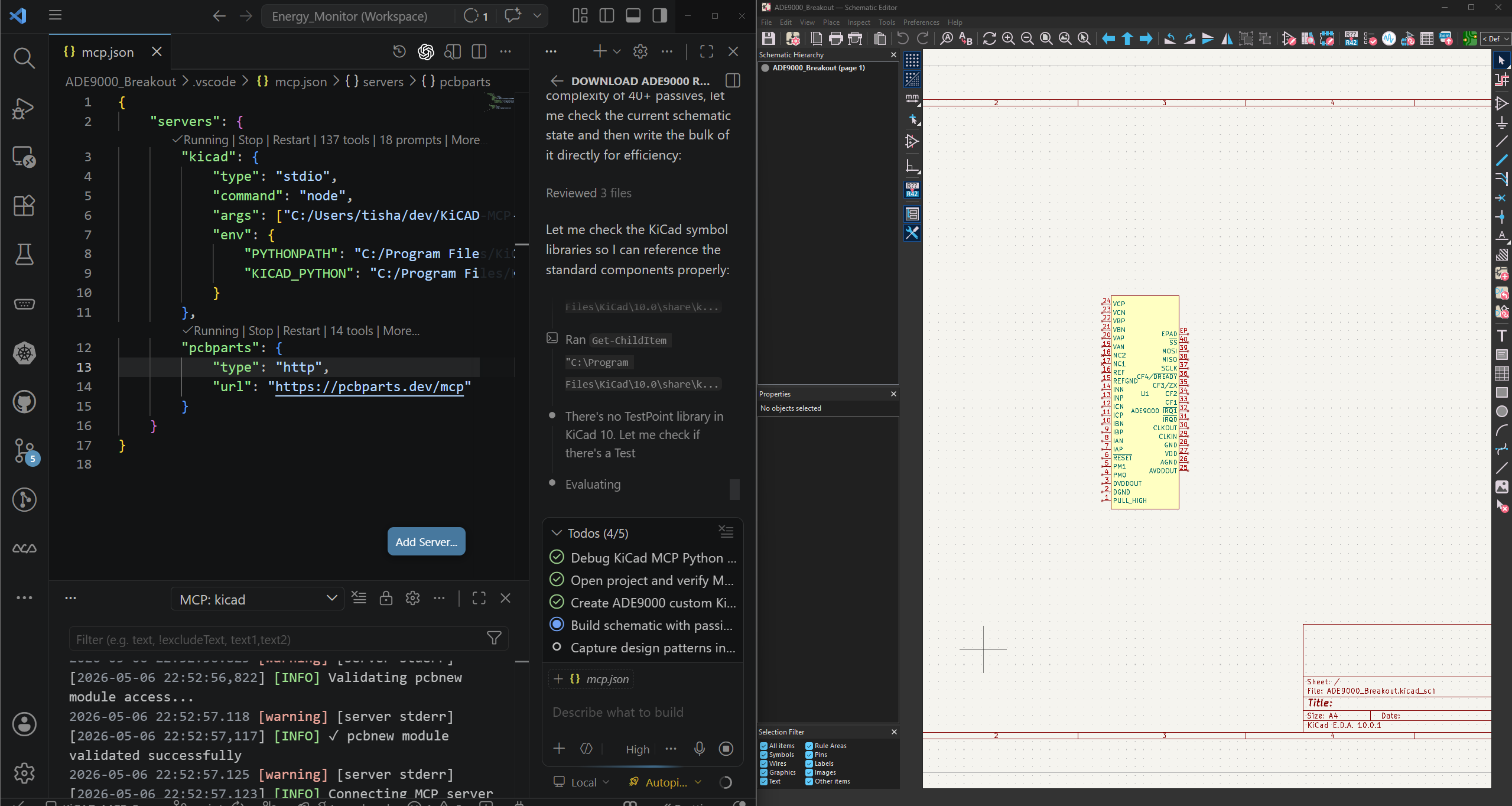
Over the last week I have been building out an ADE9000 breakout with an AI-assisted workflow wrapped around KiCAD scripting. The results are useful, occasionally impressive, and still very far from “hands-off” for precision energy monitoring.

If you grew up with “don’t trust the autorouter” as muscle memory, good news: the saying still holds. We just scaled the blast radius from one menu click to an entire AI pipeline.

What changed on the board, not just on a slide deck

The recent commit sequence in ADE9000_Breakout tells the story better than any marketing copy:

• d1e3352 (2026-05-07): “Initial AI Creation”
• 043161c (2026-05-08): “Complete routing”
• b8c8132 (2026-05-09): “Reroute with JST connector for SPI”
• a469246 (2026-05-09): “Move decoupling closer”
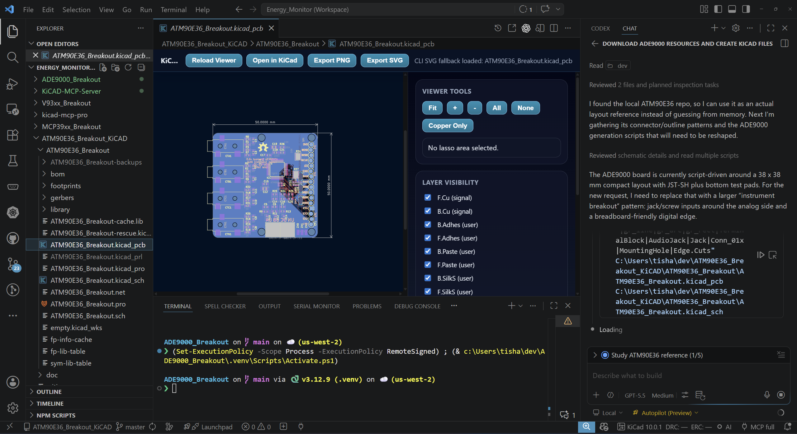
• 84b86e7 (2026-05-12): “Relayout using connectors for analog inputs”
• 7d4b420 (2026-05-16): “Rerouted with Groundplanes and new skills”
• c40e40a (2026-05-16): “Added License”
• 9b2d97e (2026-05-17): “Add project-local 3D CAD assets”
• cf8ba2c (2026-05-17): “Fix CT jack STEP orientation”
• f5a11b2 (2026-05-17): “Remove CT jack pad overlays”

This was not a single-shot generation. It was iterative engineering with scripting and machine assistance in the loop:

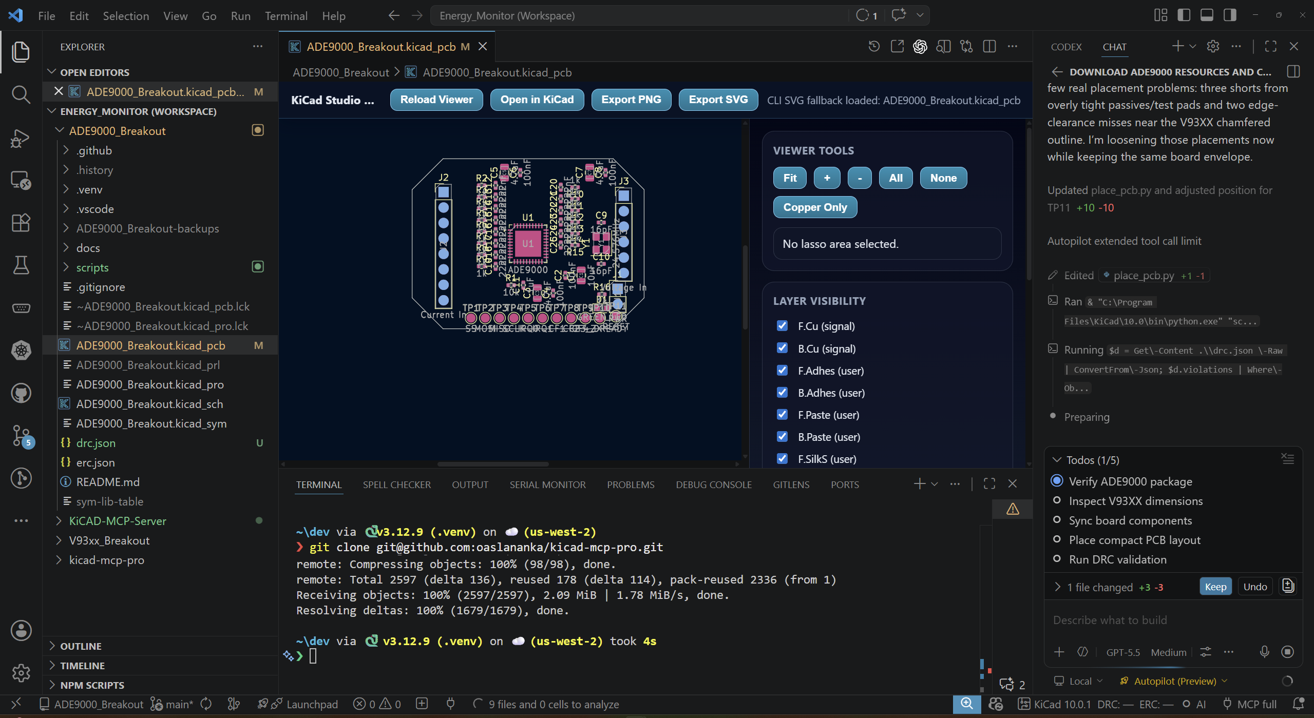
• Placement and connector mapping in scripts like place_pcb.py.
• Deterministic route passes in route_pcb.py.
• Critical route seeding and patching in seed_critical_routes.py and patch_remaining_routes.py.
• Mechanical/silk cleanup with apply_board_markings.py and move_refs_to_silkscreen.py.
• Continuous ERC/DRC artifacts (erc.json, drc.json) committed as hard checkpoints.
• 3D STEP model handling pushed into the reusable layout and size-shape skills so mechanical review can keep pace with PCB edits.

That pattern matters. The AI and automation stack gave speed and repeatability, but the engineering value came from repeated correction passes driven by board physics.

The same iteration loop is now visible in whatnick-energy-monitor-skills:

• 335a718 (2026-05-16): Initial whatnick energy monitor skills
• 78bfc44 (2026-05-17): Document STEP model workflow
• 79d925d (2026-05-17): Clarify connector STEP model matching
• af57c2d (2026-05-17): Document connector CAD alignment workflow
• 32adeff (2026-05-17): Correct ADE9000 jack CAD guidance
• d4167f6 (2026-05-17): Remove ADE9000 jack overlay guidance

That repo now captures reusable circuit, layout, routing, and board-shape guidance, plus the ADE9000 project overlay. The 3D model side was not a first-pass success either. STEP exports and connector models took multiple iterations before the project-local paths, model matching, and export workflow were stable enough to trust in a mechanical review. The later commits are the best evidence: first add local CAD assets, then discover the CT jack STEP orientation is wrong, then remove pad overlays that made the model look plausible while hiding the fact that the footprint and mechanical story needed to line up properly.

This is where AI-assisted hardware feels different from AI-assisted code. In software, a bad abstraction usually fails in tests or production logs. In PCB work, a bad abstraction can become a connector body floating neatly above the wrong pads in the 3D viewer. It looks professional right up until the part, enclosure, or cable says otherwise.

NotebookLM research: good at methodology, weaker on analog edge cases

I started on this adventure with posts from Samuel Beek promoting AI PCB design. I blended in my research background and curated a set of academic papers on AI/Algorithm usage in PCB place-n-route. I queried my pre-created NotebookLM notebook “PCB Place and Route Algorithms” specifically for mixed-signal energy-monitoring constraints.

The useful part of that synthesis:

• Current AI placement/routing research still optimizes mostly for geometric proxies (wirelength, overlap, congestion).
• Newer approaches improve constraint capture and collaboration, but are explicitly human-in-the-loop.
• Model quality degrades on low-frequency pattern classes and novel interface combinations (cold-start behavior).

The important caveat from the same query was even more telling: source coverage was strong on AI placement methodology, but thinner on precision metering specifics like safety creepage strategy, return-current choreography around split references, and “what actually ruins ENOB on a real board at 2am”.

That gap is exactly the point.

Schematik, SnapMagic, and the new hardware workflow stack

Samuel Beek’s Schematik story is almost too perfect as an origin myth for this moment. An AI-generated wiring guide for a home-grown door opener took out the fuses in his apartment, which is a fairly direct way for physics to reject your prompt. Schematik has since raised $4.6 million from Lightspeed Venture Partners and is positioning itself as a “Cursor for Hardware”: describe a device in plain language, get a bill of materials, purchase links, and assembly instructions.

The interesting engineering choice is the safety boundary. Schematik is deliberately aiming at low-voltage circuits, typically 3-5 V IoT and maker projects, because that is where the promise is large and the downside can still be bounded. That is a sensible line. It is also a reminder that “AI for hardware” is not one market. The assistant that helps someone build an MP3 player is not the same system I would trust near mains metering, isolated sensing, or a DIN rail enclosure without a lot more constraint machinery around it.

SnapMagic is attacking a nearby but different layer of the stack. Its pitch is an AI copilot for electronics design, built on the huge CAD model base that started as SnapEDA: symbols, footprints, 3D models, part discovery, BOM optimization, supply-chain substitution, and integration with existing EDA tools including KiCad. That matters because a surprising amount of PCB time is not heroic analog insight; it is finding the right model, importing it cleanly, checking whether the footprint is sane, and making sure the thing still exists at Mouser or Digi-Key.

Schematik is closer to natural-language project generation. SnapMagic is closer to CAD-data and component-selection acceleration. My little ADE9000 workflow sits in the garage between them: NotebookLM for research synthesis, KiCad Python for deterministic changes, Freerouting for a first pass, project-local skills for repeatable domain knowledge, and human review for the parts that still smell like physics.

That is the practical opening for individual designers. You do not need to wait for one perfect vendor platform. You can build a small, opinionated workflow from pieces you already control:

1. Put your design rules and recurring board-family choices into a local skill or checklist.
2. Use AI for datasheet digestion, net naming, script generation, and alternative exploration.
3. Keep KiCad, ERC, DRC, STEP export, and git history as the accountability layer.
4. Treat external libraries like SnapMagic/SnapEDA as accelerators, then verify footprints, symbols, pin numbers, and 3D models against datasheets and mechanical reality.
5. Let autorouters and AI propose routes, but hand-check return currents, decoupling loops, creepage, clocks, testability, and enclosure fit.

That sounds less magical than “hardware Cursor”, but it is much closer to how individual designers can safely get leverage today.

Why this hurts more on energy monitoring boards

An ADE9000-style board is not just “digital plus some analog”. It is a negotiated peace treaty between:

• tiny differential analog signals,
• noisy clocks and digital SPI edges,
• shared ground structures,
• high-voltage interfacing constraints,
• and assembly realities.

AI can route what it can score. Physics punishes what you forgot to score.

For energy monitoring, the failure modes are often subtle first and expensive later:

• A seemingly short route with a terrible return path becomes an EMI antenna.
• “Close enough” decoupling in XY turns into high loop inductance in 3D.
• Digital fanout convenience leaks noise into the measurement front end.
• Clearance passes in one view while creepage silently fails along real surfaces.

The scaled-up autorouter adage

Classic autorouter distrust was about ugly traces and cleanup effort.

AI-assisted distrust is about false confidence.

You now get cleaner visuals, plausible routing, and confidence scores. The board can look more “engineered” while still violating analog intent. That is worse than obviously bad output, because it delays the moment when a human gets suspicious.

In the ADE9000_Breakout commits, that showed up as repeated topology and placement adjustments:

• decoupling moved closer,
• connector strategy revised,
• critical nets explicitly seeded,
• remaining logical gaps patched after freeroute import,
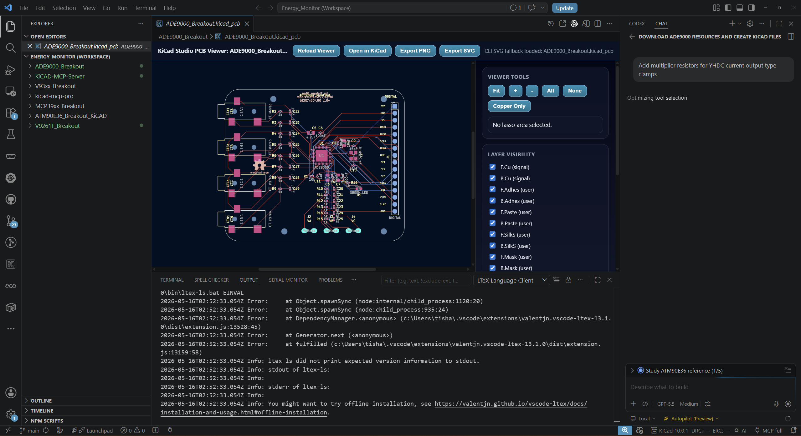
• then relayout for analog input connector realism.

None of that is anti-AI. It is pro-accountability.

A practical review checklist I now treat as mandatory

Before I trust an AI-assisted pass on a precision board, I manually review:

1. Return current continuity under each critical signal path.
2. Analog/digital ground interaction at the exact stitch points, not just net names.
3. Decoupling loop geometry (pin, cap, via topology), not just nearest-component distance.
4. Clock and fast digital net proximity to high-impedance analog channels.
5. Creepage and clearance across real isolation boundaries and along surfaces.
6. Testpoint access and assembly risks (reworkability, tombstoning, awkward probe points).

If any of those rely on “the model probably understood that”, I assume it did not.

What AI is genuinely good for in this workflow

After using it in anger, the wins are real:

• Faster exploration of placement variants.
• Deterministic scriptable edits to keep design intent reproducible.
• Constraint management that catches obvious misses early.
• Better ergonomics for repeated board evolutions.
• Mechanical and export workflows, including STEP models, can be standardized, but they still need several passes to reconcile footprint libraries, connector variants, and CAD export paths.

This is similar to CNC in machining. You still need a machinist mindset. You just get to fail faster and with better logs.

The part that still needs engineers

The physics does not care whether a trace came from a human, an RL policy, or a nicely branded copilot.

Energy metering boards live or die on the details that are hardest to encode as generic reward functions. The edge where analog integrity, EMC, and safety overlap is still mostly tacit knowledge earned through measurements, bring-up scars, and post-mortems.

So yes, use AI aggressively for PCB work. I certainly am.

Just keep the old sign above the bench.

Don’t trust the autorouter.

Now it applies to systems, not just traces.

If you are building similar mixed-signal boards, I would love to compare review checklists and failure cases that escaped DRC but showed up on the bench.

Two Agents, One Codebase: An F1 Race Team Approach to Porting ACOLITE to Rust

In Formula 1, every team fields two drivers. Not as a backup plan – as a strategy. One driver pushes the pace, forcing rivals to respond. The other holds position, manages tyres, and covers the alternative strategy. They share telemetry, they share a garage, but they are running different races on the same track. The team wins when both cars score points, not when one driver tries to do everything.

Porting a scientific Python codebase to Rust feels remarkably similar. You need the aggressive driver – the one who charges into unfamiliar code and lays down fast laps of Rust implementation. And you need the calculating driver – the one who reads the data, watches for degradation, and calls out when the numerical precision is drifting. Two AI coding agents, paired like Norris and Piastri, sharing a codebase but operating on different parts of the problem.

The Starting Grid: Why Rust for ACOLITE?

ACOLITE is RBINS’ atmospheric correction toolkit for aquatic remote sensing. It handles everything from Landsat and Sentinel-2 to hyperspectral sensors like PACE OCI (286 bands) and PRISMA (239 bands). The Dark Spectrum Fitting (DSF) algorithm is elegant – image-based, no external atmospheric inputs – but in Python, processing a full PACE scene involves reading 291 NetCDF variables, interpolating multi-dimensional LUTs, and correcting each pixel’s reflectance through a chain of gas transmittance, Rayleigh scattering, and aerosol models. On a decent machine, this takes around 230 seconds.

The seed was planted at FOSS4G 2025 in Auckland when Leo Hardtke ran a tutorial on Earth Observation processing with Rust. It was plagued by Nix environment issues (as I noted in my conference write-up), but when the code ran, it was fast. Zero-cost abstractions and fearless concurrency are not just slogans at that point – they are wall-clock seconds you are not spending waiting for your atmospheric correction to finish.

I had also been watching Rob Woodcock’s acolite-mp branch, which tackled the same performance problem from within Python. His approach was clever: per-band parallelism with memory budgets tuned to cloud CPU-to-RAM ratios (2, 4, or 8 GiB per core), replacing NumPy’s interpolation with the multithreaded pyinterp, and carefully managing the GIL contention that Python’s threading model inflicts on you. He got Sentinel-2 from 791s down to 197s and Landsat from 312s to 99s on a 24-core i9 – roughly a 3-4x speedup.

But the GIL is still there. The memory model is still Python’s. And as Rob himself noted, “further performance improvements are possible but require more extensive changes to the file handling” and “there is a fair amount of GIL contention which limits threading being caused by some structural choices in the implementation.” At some point, you are fighting the language rather than the problem.

Rust sidesteps all of this. No GIL. No garbage collector. Rayon gives you data-parallel iterators that map across bands or tiles with work-stealing. Memory usage is deterministic and known at compile time – you can profile it statically before deploying, which is a sentence that makes no sense in Python-land but is table stakes in systems programming.

The Pit Crew: Two Agents via ACP

Here is where the teammate analogy really kicks in. In F1, a team with only one driver is not half a team – it is no team at all. You cannot run a split strategy with a single car. You cannot use one driver to hold up a rival while the other pulls a gap. The performance of the pair exceeds the sum of the individuals because they create options that a solo driver simply cannot.

Porting 40,000+ lines of scientific Python to Rust is the same. A single AI agent writing Rust will drift – the implementation slowly diverging from Python’s numerical behaviour until your reflectance values are off by just enough to be scientifically useless. You need the second driver to keep it honest.

The solution I landed on was a multi-agent orchestration harness using the Agent Client Protocol (ACP), a JSON-RPC 2.0 protocol over NDJSON stdio that lets coding agents communicate in a structured way:

Agent	Role	F1 Equivalent
Kiro	Executor – writes Rust code, runs tests, reads files	Lead driver – pushes the pace, sets fast laps
Copilot	Proposer – reviews output, suggests next steps, cross-checks Python	Second driver – covers the strategy, watches the gaps
Human	Approver – filters proposals before dispatch	Team principal – makes the call on when to pit

The workflow per sensor port looks like this:

1. Human provides --task to the orchestrator (tools/agent_harness.py)
2. Kiro receives the task via ACP session/prompt and starts writing code
3. Kiro streams output via session/update chunks
4. Output goes to Copilot for review against the Python source
5. Copilot proposes ACTION: lines – “fix the gas transmittance interpolation order”, “the Rayleigh LUT needs pressure stacking”
6. Human approves or rejects
7. Approved actions go back to Kiro
8. Repeat until regression tests pass or maximum cycles reached

This is not vibe coding. This is a two-car team running a split strategy.

Think about how McLaren or Red Bull operate. The lead driver qualifies on pole and sets the pace in clean air. The second driver starts on a different tyre compound, runs a longer first stint, and emerges from the pits into a different part of the field. They are solving complementary problems – one optimises for raw speed, the other for strategic coverage. Neither is redundant.

Kiro is the lead driver. It attacks the Rust implementation aggressively – writing loaders, porting DSF algorithms, wiring up rayon parallelism. It sets fast laps. It also occasionally bins it into the gravel trap by hallucinating a NumPy broadcasting rule that does not exist in ndarray.

Copilot is the second driver. It reads the Python source, cross-references the Rust output, and spots where the gap to parity is growing. “The gas transmittance interpolation order is wrong” is exactly the kind of radio call a second driver makes – not flashy, but it prevents a DNF.

The human is the team principal. You do not override the drivers on every corner, but you make the strategic calls: do we pit now and fix this RMSE regression, or do we push on and address it in the next stint? Is a 0.002 RMSE difference in Sentinel-2 reflectance acceptable? (It is – that is within float32 precision.) When do we switch from tiled DSF to fixed DSF mode for this sensor?

Together, they converge faster than either alone, for the same reason that two cars gathering tyre data in free practice gives the team more information than one car doing twice as many laps.

The Telemetry: Regression Tests Against Real Data

In F1, both drivers generate telemetry. The team overlays their data – braking points, throttle application, cornering speed – to find where one is faster and why. The overlay is the truth. Not the driver’s feeling, not the engineer’s simulation, but what the car actually did on the track.

Regression tests are our telemetry overlay. The Python ACOLITE output is Driver 1’s trace. The Rust output is Driver 2’s. We overlay them pixel-by-pixel, band-by-band, and look at the delta. When the traces diverge, something real has changed and we need to understand whether it is a genuine improvement or an error we need to correct.

There are currently 141 Python regression tests that compare Rust output against Python output pixel-by-pixel across real satellite scenes:

• Landsat 8/9: 13 regression + 13 Rust-vs-Python + 7 benchmark tests
• Sentinel-2 A/B: 19 regression + 15 Rust-vs-Python + 9 benchmark tests
• PACE OCI: 17 regression + 14 Rust-vs-Python + 12 DSF comparison + 12 ROI + 10 full-scene tests

The tolerances are tight. Sentinel-2 achieves RMSE < 0.002 (physics-equivalent). Landsat gets RMSE < 0.02. PACE full-scene (1710 x 1272 pixels x 291 bands) hits mean RMSE of 0.004 with 100% of pixels within 0.05 of Python. Correlation coefficients are R > 0.999 across all sensors.

These are not toy tests on synthetic data. They run against actual L1 scenes downloaded from USGS and NASA. When the tests break, something real is wrong.

The Performance Gap: Where the Seconds Go

Sensor	Scene Size	Rust	Python	Speedup
Landsat 8	62M px x 7 bands	66s	180s	2.7x
Landsat 9	62M px x 7 bands	56s	180s	3.2x
Sentinel-2 A	30M px x 11 bands	52s	182s	3.5x
Sentinel-2 B	30M px x 11 bands	64s	173s	2.7x
PACE OCI (full)	1710 x 1272 x 291 bands	84s	230s	2.7x

The PACE result is particularly satisfying. The key optimisation was switching from 291 per-band NetCDF reads to 3 bulk detector reads, then applying rayon-parallel atmospheric correction across tiles. Load is 12 seconds, AC is 34 seconds, write is 35 seconds. That write phase for a 291-band hyperspectral cube goes to GeoZarr V3 with gzip compression – try doing that in a Python event loop without your memory allocator throwing a tantrum.

Energy Efficiency: The Fuel Strategy Nobody Talks About

Here is the part where I get philosophical – and where the F1 analogy turns from metaphor into mirror.

Formula 1 underwent a fuel efficiency revolution in 2014. The FIA introduced hybrid power units, capped fuel flow at 100 kg/hour (monitored 2,200 times per second), and forced teams to extract maximum performance from minimum fuel. The result was not slower cars – it was faster cars that used less. The 2026 regulations go further: fossil carbon is prohibited entirely, the MGU-K will deliver three times the electrical power (350kW vs today’s 120kW), producing up to 1,000 horsepower while burning sustainable fuel. Less fuel, more power. That is not a trade-off – it is an engineering constraint that drives innovation.

The same constraint applies to scientific computing, we just pretend it does not. Cloud computing bills are denominated in dollars, but the underlying unit is energy. Every CPU cycle your atmospheric correction burns is a watt drawn from a power grid somewhere. When you are processing continental-scale Sentinel-2 archives or the full PACE ocean colour mission, those watts add up. Python is the V10 era of scientific computing – glorious, unrestricted, and profligate with resources.

Rust is the hybrid power unit. Its advantage is not just speed – it is energy per unit of work. A 3x speedup roughly translates to using a third of the compute time, which means a third of the energy, a third of the carbon footprint, and a third of your AWS bill. The Rust Foundation and others have pointed to studies showing compiled languages like Rust and C using an order of magnitude less energy than interpreted languages for equivalent workloads. Just as F1 teams discovered that fuel efficiency constraints forced them to build fundamentally better engines, switching to Rust forces you to think about memory layout, allocation patterns, and data flow in ways that Python’s garbage collector lets you ignore – until the bill arrives.

And here is the irony that would make an F1 sustainability officer wince: Earth observation processing is meant to monitor the planet’s health. Burning excess energy to do it is like running your emissions-monitoring car on leaded fuel. F1 recognised that the sport’s 20-car grid is only 1% of its total carbon footprint, but pursued fuel efficiency anyway because the technology trickles down. The same logic applies to EO processing pipelines. The individual savings per scene are modest, but at continental archive scale they compound – just like how F1’s hybrid innovations now power road cars from Ferrari’s SF90 to the electric components in every modern turbo engine.

Static memory profiling makes this tangible. In Rust, I can tell you at compile time that a Sentinel-2 full-scene atmospheric correction will peak at approximately N gigabytes of memory, because the allocations are deterministic. In Python, you find out at runtime – usually when the OOM killer visits your pod. F1 teams know their fuel load to the gram before the formation lap. Rust gives you the same certainty for compute.

Kubernetes 1.35 and Vertical Pod Autoscaling

This deterministic memory behaviour dovetails nicely with Kubernetes 1.35’s improvements to Vertical Pod Autoscaler (VPA). VPA watches your pod’s actual resource usage and adjusts CPU and memory requests/limits accordingly. When your workload has predictable resource usage – as Rust workloads tend to – VPA converges quickly to the right allocation instead of oscillating between OOM kills and wasted headroom.

For a processing pipeline that ingests satellite scenes of varying sizes (a Landsat scene is 62 million pixels across 7 bands; a PACE scene is 2.2 million pixels across 291 bands), VPA can right-size pods per sensor type. Rust’s static memory profile means the VPA recommendations stabilise fast, which means tighter bin-packing, which means more scenes processed per node, which means lower cost per scene.

Compare this to Python pods where memory usage is non-deterministic, garbage collection spikes are unpredictable, and the VPA has to overprovision to avoid OOM. The 2 GiB/core cloud ratio that Rob’s acolite-mp was carefully designed around becomes less of a constraint when your language does not waste half of it on interpreter overhead.

Out-of-Band Development: Preventing Merge Conflicts with Upstream

One design decision I am particularly happy with is keeping the Rust port on a separate feature branch (feature/rust-port) and treating it as out-of-band from the Python codebase. ACOLITE upstream is actively maintained by Quinten Vanhellemont at RBINS, with regular additions of new sensors, algorithm refinements, and bug fixes. A traditional “rewrite in Rust” approach would create an immediate fork that diverges with every upstream commit.

Instead, the Rust code lives in src/, benches/, and tests/ directories that do not exist in upstream Python ACOLITE. The Python code in acolite/ stays untouched. The regression tests are the synchronisation mechanism – they import both the Python ACOLITE modules and the compiled Rust binary, run the same scene through both, and compare outputs.

When upstream adds a new sensor or changes a gas transmittance coefficient, the regression tests fail in the Rust port. That failure is the trigger: it goes into the agent harness as a --task, Kiro investigates the numerical difference, Copilot cross-references the upstream commit, and the fix lands in Rust without touching a single Python file. No merge conflicts. No rebasing nightmares. Just tests that enforce parity.

This is how you keep an acceleration layer in sync with a moving target – you do not try to merge them. You test them against each other.

What Is Next: The Gap to Full Sensor Parity

The roadmap has the current state at 48 Rust tests, 141 Python regression tests, and three sensors fully validated (Landsat 8/9, Sentinel-2 A/B, PACE OCI). The architecture – loader, AC, writer – is clean and extensible. But three sensors out of 30+ is a qualifying lap, not a race win. Here is what closing the gap to full ACOLITE parity actually looks like.

Sensor Coverage: 3 down, 30+ to go

Python ACOLITE supports a sprawling constellation of sensors. The Rust port has ticked off the three highest-priority ones but the remaining fleet breaks into tiers:

Tier 1 – Near-term (shared loader patterns exist):

Sensor	Bands	Loader Type	Blocker
Sentinel-3 OLCI	21	NetCDF	Sensor def exists, needs full pipeline
PRISMA	239	HDF5	Shares pattern with PACE
DESIS	235	HDF5	Shares pattern with PACE
EnMAP	224	HDF5	Shares pattern with PACE
EMIT	285	NetCDF	Similar to PACE OCI

These are the low-hanging fruit. The PACE port proved out the NetCDF and hyperspectral GeoZarr writer path; PRISMA/DESIS/EnMAP share the HDF5 loader pattern. Each is a well-scoped --task for the agent harness – Kiro writes the loader and wires up the AC pipeline, Copilot validates against Python output on a reference scene.

Tier 2 – Medium-term (new loader work required):

Sensor	Bands	Notes
Landsat 5 TM / 7 ETM+	7-8	Older calibration metadata formats
PlanetScope (Dove/SuperDove)	4-8	Commercial format, GeoTIFF based
WorldView-2/3	6-29	Multi-resolution, pan-sharpening
Pleiades	5-7	DIMAP format
QuickBird-2	5	Legacy but still used
VIIRS (NPP/J1/J2)	22	Swath-based HDF5, three platforms
Aqua/Terra MODIS	36	HDF4/HDF-EOS
GOCI-2	12	Korean ocean colour mission

Each of these needs a dedicated loader – different metadata formats, different calibration approaches, different file layouts. The atmospheric correction core (DSF, gas transmittance, Rayleigh, aerosol models) is shared, but getting the radiometrically calibrated top-of-atmosphere reflectance array into the pipeline is the per-sensor work.

Tier 3 – Geostationary and niche (lowest priority for aquatic applications):

GOES ABI, Himawari AHI, MTG-I FCI, SEVIRI, Sentinel-3 SLSTR, AMAZONIA-1 WFI, CHRIS, HYPERION, HICO, HyperField, HYPSO, Tanager. Some of these (HYPERION, HICO) are decommissioned but their archives are still processed. Others (Tanager at 420 bands, HYPSO at 120) are newer hyperspectral missions that would benefit most from Rust’s performance advantage.

Beyond Loaders: The Algorithm Gap

Sensor parity is not just about reading files. Python ACOLITE has several processing features the Rust port does not yet implement:

• ROI subsetting: Limit processing to a bounding box or polygon – critical for operational workflows that do not need a full scene
• Ancillary data retrieval: NCEP ozone, pressure, and wind speed from NASA OBPG; currently the Rust port uses default values
• DEM-derived pressure: Copernicus DEM at 30/90m for surface pressure estimation in mountainous coastal regions
• Glint correction: Sun glint removal for low-latitude ocean scenes
• RAdCor adjacency correction: The physics-based adjacency effect correction developed under the STEREO program
• TACT thermal processing: Surface temperature from Landsat thermal bands via libRadtran – this one is architecturally interesting because it requires calling an external Fortran radiative transfer code
• Interface reflectance (rsky): Sky reflection correction at the air-water interface
• L2W water products: Chlorophyll-a (OC algorithms), TSS (Nechad, Dogliotti), turbidity, Secchi depth – the derived products that downstream scientists actually use

The L2W gap is the most consequential. Most ACOLITE users do not care about surface reflectance per se; they want chlorophyll maps or turbidity time series. Until the Rust port can produce L2W outputs, it remains a fast atmospheric correction engine rather than a complete aquatic remote sensing toolkit.

The Realistic Path

Closing this gap is not a sprint, it is an endurance race – appropriately enough. The agent harness makes each sensor port a repeatable, testable unit of work. The pattern is established: write loader, wire to AC pipeline, run regression tests against Python, fix deltas, validate on real data. Each sensor port takes the agents a day or two of focused work plus human review.

At the current pace, Tier 1 sensors are within reach in the near term. Tier 2 will follow as the loader library matures. The algorithm features (ancillary data, glint, TACT) are orthogonal to sensor coverage and can be developed in parallel. L2W is the final milestone – when the Rust port can ingest a Sentinel-2 scene and produce a chlorophyll-a map that matches Python to within measurement uncertainty, the port will be race-ready for production.

Each of these is a --task for the agent harness. Two drivers, one constructor’s championship. The lead driver pushes into unfamiliar sensor territory, the second driver validates against Python, and the telemetry overlay catches every divergence before it compounds into a retirement.

If the intersection of Rust, Earth observation, and AI-assisted development interests you, the code is all on GitHub. Feel free to ping me with ideas, bug reports, or competing approaches – especially if you have a cleverer way to handle the N-dimensional LUT interpolation. That one was a fun 3 days of Rapid Rust Rewrite fuelled by AI Amphetamine Analogs.

Rage against the machine - Pattern Matching

One of the major strengths (and sometimes weakness) of the human brain is its ability to perform pattern matching - the classic is where people play more attention while playing games and digitising and gamifying the airport security leads to less false positives. We perform heuristics in everything we see and hear, often coming to conclusions based on partial information, based on extrapolation performed using past experience. This is why upper-case letters in English are so much easier to read since we have built up heuristics to infer the letter from the top-half, people who write in all capitals seem to be almost shouting as our visual heuristics take the cue.

Ambiguous painting

Machines are getting better at the heuristics as well as brute force, we have passed them on just the way we pass on preconceptions of right and wrong, beauty and religion to our children. Based on this system of thought and accumulated body of knowledge, machines can perform pattern matching tasks they are programmed for in vastly superior ways than humans. All they demand in return is energy, materials to build them and intelligent human beings to make some long intellectual marches in programming them.

Cat videos are the dominant species

In someways the rote jobs of pure pattern matching has made us mental Neanderthals with short neural loops focused on ambush hunting only the job at hand, rather than thinking long term strategy. The long chase where all the short easy pattern matching jobs have been mechanised is for the more creative, the artists. Yet there is still need for the engineer to keep the machines functioning. There are always predictions of race of against the machines. We still need to communicate our mental models imperfectly via whatever means.

Genies are just machines with Genius

May be with exposure to lots of cat videos and artwork, the machine will eventually learn to play with cats while painting, and we will keep building bigger machines since we can't be born biologically with bigger skulls or weild GeV's with our finger tips.